Specialized Data Stores: Redis, Elasticsearch, Cassandra, Neo4j & Vector Databases
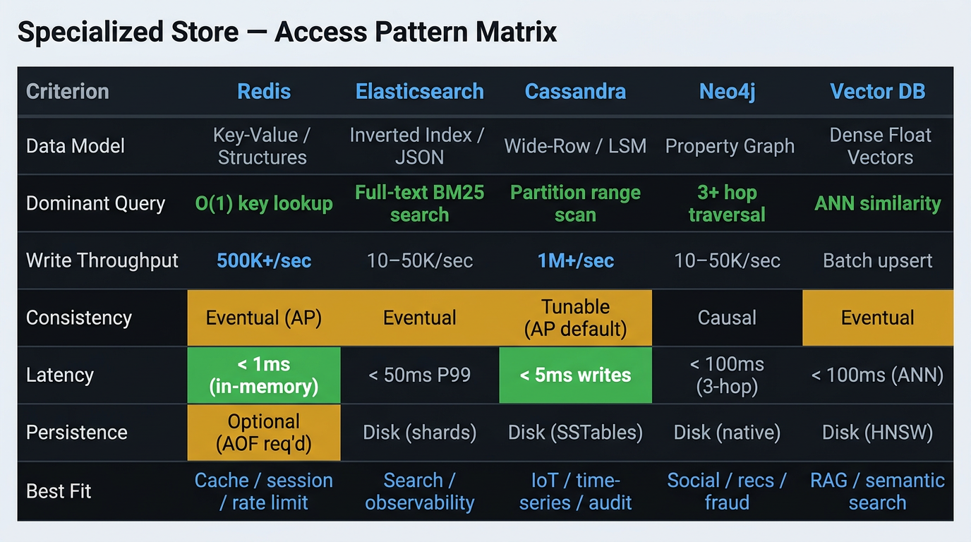
Specialized data stores are purpose-built acceleration layers — each solves an access pattern that general-purpose databases serve poorly. This article covers Redis persistence trade-offs, Elasticsearch inverted index mechanics, Cassandra's LSM-tree write path, Neo4j graph traversal, and a beginner-level introduction to vector databases and ANN search.
Modern Database Paradigms
Specialized Data Stores: Redis, Elasticsearch, Cassandra, Neo4j & Vector Databases
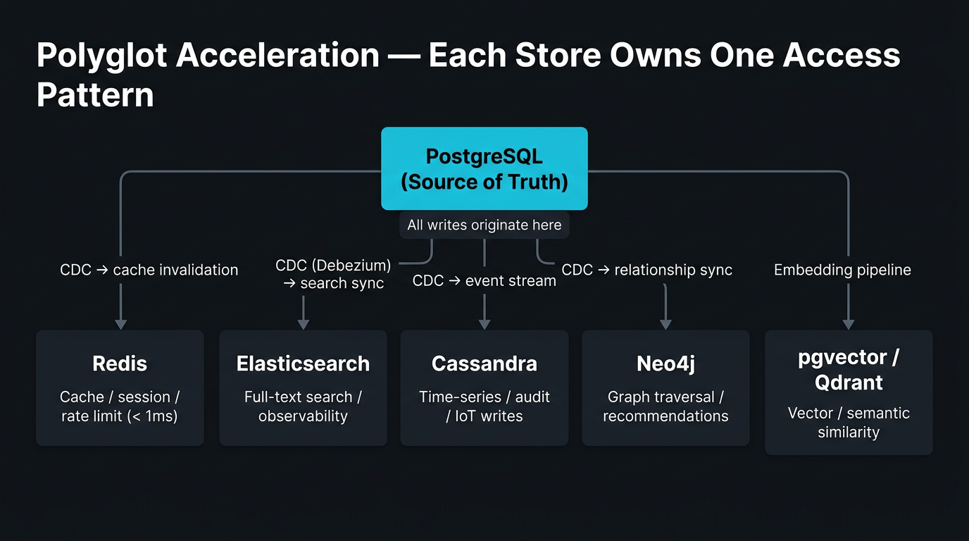
Selecting the right database is a foundational architectural decision; data gravity ultimately dictates the scalability and resilience of an application — choose the paradigm first, the product second. The broken pattern for specialized stores is adopting them by category rather than by access pattern: "we need caching, so Redis"; "we need search, so Elasticsearch"; "we need a graph, so Neo4j." Each of these stores has a canonical failure mode that appears when it is used for the wrong workload — and a canonical strength that makes it orders of magnitude better than a general-purpose database for the right one. This article covers all five stores, their mechanics, their data modeling discipline, their failure modes, and the precise conditions under which each is justified.
Redis — From Cache to Architectural Store
Architecture
Redis is a single-threaded, in-memory data structure server. Its performance comes from two sources: all data in RAM (no disk I/O on reads) and a non-blocking I/O event loop that processes thousands of commands per second on a single thread.
Data Structures and Use Cases
| Structure | Command Pattern | Production Use Case |
|---|---|---|
| String | SET key value EX ttl |
Cache, idempotency keys, feature flags |
| Hash | HSET session:userId field value |
Session objects (field-level GET/SET) |
| Sorted Set | ZADD leaderboard score userId |
Leaderboards, rate limiting windows |
| List | LPUSH queue task; RPOP queue |
Work queue, activity feed |
| Set | SADD online:users userId |
Unique visitor tracking, tag sets |
| Stream | XADD events * action login userId 42 |
Event sourcing, pub/sub, audit log |
Data Modeling for Redis
Redis Stack — Beyond Caching
When NOT to Use Redis
- As a primary store without AOF enabled — RDB snapshots can lose up to 60 seconds of writes on crash
- For datasets exceeding available RAM without an explicit eviction policy (
allkeys-lrufor cache-only workloads) - For complex relational queries or multi-entity aggregations — no join primitives
- For compliance-auditable data that must survive every crash without a durable secondary backing it
Elasticsearch / OpenSearch — Full-Text Search and Observability
Inverted Index Mechanics
SQL LIKE '%keyword%' requires a sequential scan of every row. The inverted index maps tokens to document IDs in O(1) — this is why Elasticsearch retrieves relevant results in milliseconds across billions of documents.
Data Modeling for Elasticsearch
"dynamic": "strict" causes Elasticsearch to reject documents with unmapped fields, preventing mapping explosion. Mapping explosion (thousands of dynamic fields from log data) bloats the cluster state, triggers GC pauses, and is the most common Elasticsearch production incident. Always set dynamic: strict in production indexes.
Index Lifecycle Management
When NOT to Use Elasticsearch
- As a primary database — no ACID guarantees, no foreign keys, writes are eventually indexed
- For transactional writes requiring sub-5ms acknowledgment — Lucene indexing adds overhead
- For small datasets (< 1M documents) — Postgres
tsvectorwith a GIN index is operationally simpler and sufficient
Apache Cassandra — Write-Optimized Distributed Storage
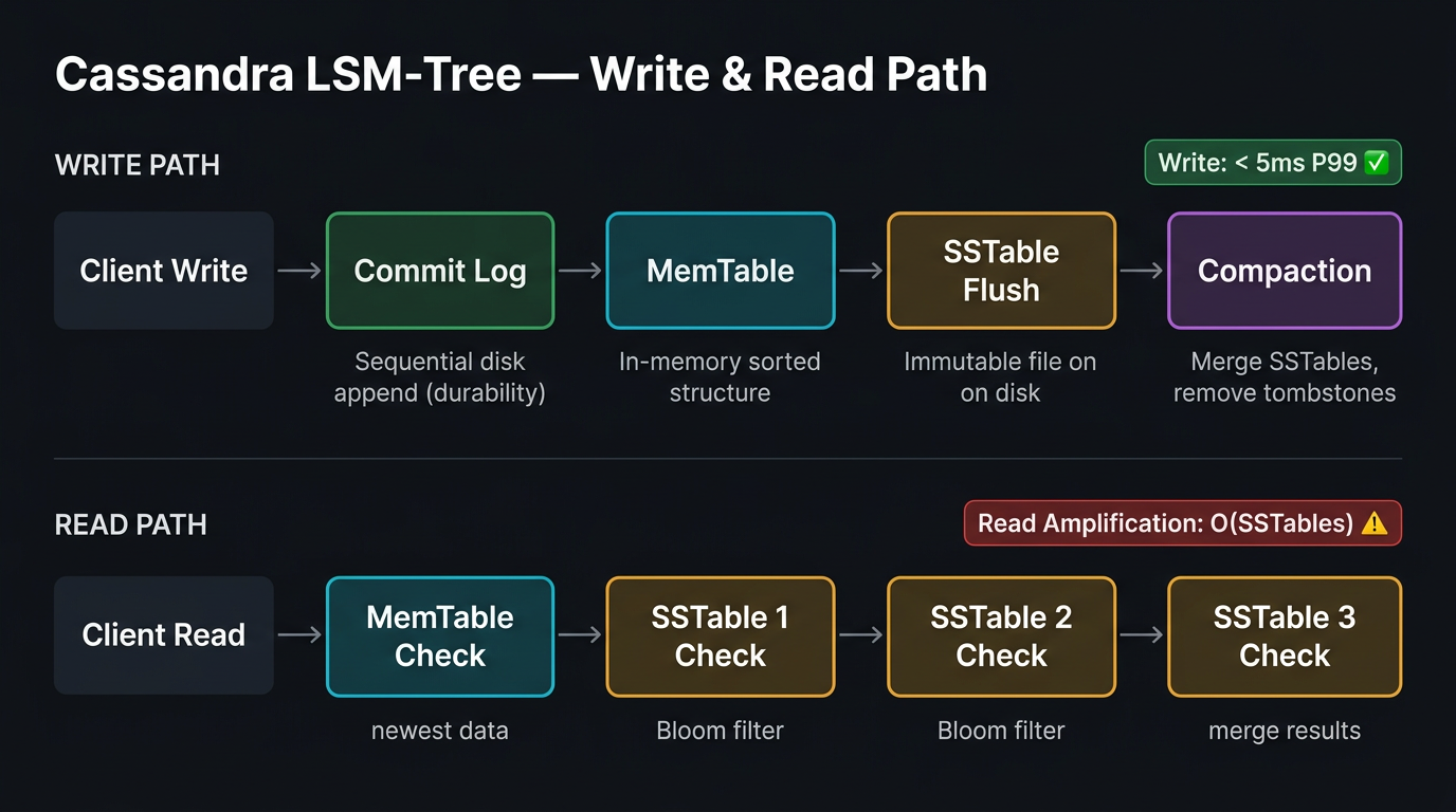
LSM-Tree Write Path
The implication: Cassandra is optimized for writes that are never updated. A workload that frequently updates individual records creates read amplification and compaction pressure — the wrong fit for an LSM-tree.
Data Modeling for Cassandra
GDPR Compliance: Cassandra's LSM-tree and distributed replication make immediate physical erasure impossible. A DELETE statement writes a tombstone — the actual data persists in SSTables until compaction completes, which may take hours or days across replicas. Design a compliance strategy upfront: use TTL (expiry, not erasure) for time-bounded data, and encryption-key-deletion for immediate logical erasure of PII. Document this strategy before your first compliance audit — "we deleted it" is not sufficient if the data exists in SSTables.
Compaction Strategies
| Strategy | When to Use | Anti-Pattern |
|---|---|---|
| STCS (SizeTieredCompactionStrategy) | Write-heavy workloads with infrequent reads | Time-series — causes unbounded SSTable growth |
| LCS (LeveledCompactionStrategy) | Read-heavy workloads requiring predictable latency | High write throughput — compaction cannot keep up |
| TWCS (TimeWindowCompactionStrategy) | Time-series, IoT, append-only with TTL | Any workload with frequent overwrites to the same key |
When NOT to Use Cassandra
- Read-heavy workloads with random point-access — read amplification across SSTables degrades P99
- Workloads requiring complex aggregations — Cassandra has no aggregation primitives beyond
COUNTandSUMper partition - Small teams without JVM expertise — compaction tuning, GC pressure, and tombstone monitoring require operational depth
Neo4j — Graph Database for Connected Data
Property Graph Model
Data Modeling for Neo4j
When NOT to Use Neo4j
- Tabular reporting where rows are filtered by properties, not traversed by relationships
- High-volume transactional writes — graph locking on shared nodes degrades throughput at Cassandra/DynamoDB write rates
- Workloads with no meaningful multi-hop relationship traversal — if queries don't follow edges, it is a relational dataset in a graph store
Vector Databases — Beginner Introduction
What Is an Embedding?
ANN — Why Approximate Search Is Necessary
Exact nearest neighbor search across 10M 1536-dimension vectors requires computing 10M cosine distances per query — O(n×d) time where d is the dimension count. At 10M vectors and 1536 dimensions, this is ~15 billion float multiplications per query — approximately 10 seconds on a single CPU core.
HNSW (Hierarchical Navigable Small World): builds a multi-layer graph where each node links to its nearest neighbors. Queries traverse from sparse upper layers to dense lower layers — finding approximate nearest neighbors in O(log n) time with high recall.
IVFFlat (Inverted File with Flat quantization): clusters vectors into nlist buckets at training time. Queries search only the top nprobe closest buckets — fast, but recall degrades if the query vector's neighbors span multiple buckets.
The RAG Pipeline
Start with pgvector inside your existing Postgres instance. It eliminates a separate infrastructure dependency, supports HNSW and IVFFlat indexes, enables hybrid queries (vector similarity + SQL filters in one query), and handles under 10M vectors at sub-100ms P99 on modern NVMe hardware. Graduate to Qdrant or Pinecone when retrieval P99 consistently exceeds your latency budget.
Cost Model at Scale
| Store | Config | 1M ops/day | 10M ops/day | 100M ops/day |
|---|---|---|---|---|
| Redis | ElastiCache r6g.large | ~$50/mo | ~$120/mo | ~$500+/mo |
| Elasticsearch | OpenSearch t3.medium.search | ~$50/mo | ~$200/mo | ~$800+/mo |
| Cassandra | 3× i3.large self-hosted | ~$300/mo (fixed) | ~$300/mo (fixed) | ~$600/mo (6 nodes) |
| Neo4j | AuraDB Professional | ~$65/mo | ~$200/mo | Custom |
Cassandra's cost model is flat until you need more nodes — it scales by adding nodes, not by paying per operation. This makes it cost-effective at extreme write volumes where DynamoDB's per-request pricing would be prohibitive.
Security
| Store | Auth Mechanism | Transport | Encryption at Rest |
|---|---|---|---|
| Redis | requirepass + ACL (per-command) |
TLS (optional, enable explicitly) | Managed: enabled. Self-hosted: OS-level |
| Elasticsearch | X-Pack RBAC, field-level security | TLS mandatory (v8+) | Enabled by default (v8+) |
| Cassandra | Native auth + RBAC | TLS (node-to-node + client) | Transparent Data Encryption (TDE) |
| Neo4j | RBAC on labels/relationships | TLS (bolt protocol) | Managed: enabled. Self-hosted: OS-level |
Summary
| Concept | Rule |
|---|---|
| Redis persistence | Redis AOF persistence (appendfsync everysec) is mandatory whenever Redis stores data you cannot afford to lose — RDB alone loses up to 60 seconds. |
| Elasticsearch mapping | Elasticsearch dynamic mapping causes index bloat and query degradation — enforce explicit mappings and disable dynamic: true on production indexes. |
| Cassandra write model | Cassandra's write performance is structural (LSM-tree append-only), not configurable — never model workloads that require frequent point-read updates. |
| Neo4j graph traversal | Neo4j's Cypher is orders of magnitude faster than recursive SQL CTEs for 3+ hop relationship queries — but only when the access pattern is genuinely relational. |
| Vector database entry point | Start vector search with pgvector inside your existing Postgres stack; migrate to a dedicated vector store only when retrieval P99 exceeds your latency budget. |
Related: Database Foundations Series — Apache Cassandra is a masterless BASE store, using gossip membership, tunable quorums (LOCAL_QUORUM, ONE, ALL), and Merkle tree anti-entropy to achieve eventual consistency without a global coordinator. For the formal BASE paradigm that Cassandra implements, see BASE Database Properties: Basically Available, Soft State & Eventual Consistency.
What's Next
In Part 6, we cover polyglot persistence — how to quantify when multiple databases earn their operational cost, how Change Data Capture with Debezium replaces the dual-write anti-pattern, and when Postgres extensions eliminate entire database tiers.
This article was developed with AI-assisted deep search, specification cross-referencing, and technical research synthesis.