The Database Decision Framework: Choose the Paradigm Before the Product
Defaulting to a familiar database is an architectural mistake. This article introduces a structured decision process — workload classification, access pattern analysis, and consistency model selection — that must precede any product evaluation, plus a diagnostic checklist for ruling out application-layer bottlenecks before adding a new database.
Modern Database Paradigms
The Database Decision Framework: Choose the Paradigm Before the Product
Selecting the right database is a foundational architectural decision; data gravity ultimately dictates the scalability and resilience of an application — choose the paradigm first, the product second. The most expensive database mistake is not choosing the wrong engine — it is choosing an engine before understanding the workload. Teams that default to a familiar tool ("we use Postgres for everything") eventually reach a wall: a sharding problem Postgres cannot solve, a graph traversal that recursive CTEs cannot serve, or a write throughput ceiling that a single primary cannot absorb. This article gives you the structured decision process that prevents that wall.
1. Diagnostic Checklist — Is My Database Actually the Bottleneck?
Before adding a new database to your stack, rule out that your existing database is the problem. Most "we need a new database" decisions are actually application-layer problems in disguise.
Work through this checklist against your primary store before evaluating alternatives:
If seq_pct exceeds 10% on a table with over 100K rows, you have a missing index — not a database paradigm problem.
| Symptom | Root Cause | Fix Before Switching |
|---|---|---|
| Slow queries on large tables | Missing indexes, bad query plan | Add targeted index; run ANALYZE |
| App threads blocking under load | N+1 query pattern | Fix query at the ORM/query layer |
| Connection refused / timeout | Connection pool exhaustion | Deploy PgBouncer in transaction mode |
| High memory usage | Missing query result limits | Add LIMIT clauses; paginate |
| Write latency spike at high volume | No connection pooling on writes | PgBouncer + async write queue |
Only proceed to a new database paradigm when the bottleneck cannot be eliminated by indexing, query rewriting, connection pooling, or vertical scaling. Adding a second database before fixing the application layer compounds the problem — you now have two stores to debug.
2. Workload Taxonomy
Every database paradigm is optimized for a workload class. The first step in any database selection is classifying your own.
| Workload Class | Dominant Operation | Latency Requirement | Consistency Requirement |
|---|---|---|---|
| OLTP (Online Transactional Processing) | Point reads + writes, short transactions | < 10ms P99 | Strong (ACID) |
| OLAP (Online Analytical Processing) | Full-table scans, aggregations, joins | Seconds acceptable | Eventual or snapshot |
| HTAP (Hybrid) | Mixed OLTP + light analytics | < 50ms for OLTP path | Strong for writes, eventual for reads |
| Search | Full-text, faceted, fuzzy matching | < 50ms P99 | Eventual |
| Graph | Multi-hop relationship traversal | < 100ms for 3–5 hops | Causal or strong |
| Cache / Session | Single key lookup, TTL expiry | < 1ms P99 | Eventual (loss-tolerant) |
| Vector / Similarity | ANN search on high-dimensional embeddings | < 100ms P99 | Eventual |
| Time-Series / Append-Only | Sequential writes, range-time reads | < 5ms write P99 | Eventual |
If you can describe your workload with "mostly point reads and writes on structured entities," you have an OLTP workload. If you say "we need to find all users similar to this user" or "run this report across the last 90 days," you have a different workload class entirely.
5-minute classification: Count your top 10 queries by frequency. What fraction are point lookups (fetch by primary key or unique index)? What fraction are scans or aggregations? What fraction follow relationships across 2+ entities? The largest bucket defines your primary workload.
3. Access Pattern Analysis
Workload class narrows the field. Access patterns determine the specific paradigm.
3.1 Point Lookup
Point lookups by a known key are served equally well by relational, key-value, and document stores. The differentiator is what else you need — if the answer is "complex queries," relational wins; if "extreme write throughput," key-value or document wins.
3.2 Range Scan
Range scans favor relational databases (B-tree indexes) and Cassandra (clustering columns). DynamoDB can handle ranges but requires the full access pattern to be modeled into the table key design before the first write.
3.3 Graph Traversal
The SQL version is not just slower — it scales with O(n³) join complexity. At 10M orders, the SQL approach is not just slow; it is impractical. Graph traversal at 3+ hops is the clearest signal to use a graph database.
3.4 Aggregation
Complex, ad-hoc aggregations favor relational databases. If you can define the aggregation shape upfront, Cassandra counter tables or DynamoDB GSI projections can work — but you lose flexibility. Arbitrary aggregations require SQL.
4. Consistency Model Spectrum
Consistency is a contract between the database and the reader: what version of the data are you guaranteed to see after a write completes?
| Model | Guarantee | Latency Impact | Use When |
|---|---|---|---|
| Strong / Linearizable | Every read sees the most recent committed write | +RTT for quorum | Financial transactions, inventory, seat reservation |
| Causal | Reads see writes that causally preceded them | +small overhead | Social feeds, collaborative editing |
| Read-Your-Writes | You always see your own writes | Minimal | User profile updates, session data |
| Eventual | Reads eventually converge to the latest write | Lowest | Counters, analytics aggregates, search indexes |
5. The CAP Theorem in Practice
CAP states that a distributed system can guarantee at most two of: Consistency, Availability, Partition Tolerance. In cloud deployments, network partitions are not theoretical — they happen. Partition tolerance is non-negotiable.
This makes CAP a real-world choice between CP (consistent under partition, may reject writes) and AP (available under partition, may serve stale reads).
| Database | CAP Position | What It Means in Practice |
|---|---|---|
| PostgreSQL | CP | Under partition: primary continues; replicas may serve stale reads |
| CockroachDB | CP (serializable) | Under partition: Raft majority required for writes; minority nodes pause |
| MongoDB (majority write concern) | CP | Under partition: primary election; secondary reads may be stale |
| DynamoDB | AP (default) | Under partition: serves eventual reads; conditional writes enforce consistency |
| Cassandra | AP (tunable) | QUORUM consistency trades availability for consistency at write time |
| Redis | AP (no persistence) | Under partition: stale reads possible; data loss if primary crashes without AOF |
6. Polyglot Persistence Cost Model
Adding a second database to your stack is an operational multiplier, not just a technical decision.
Per-database ongoing cost:
Before adding a second database, answer: does the performance delta of the specialized store at my current scale exceed the fully-loaded cost of operating it? If your dataset is under 10M rows/documents/vectors, the answer is almost always no — a single Postgres instance with the right extensions outperforms the operational cost of a second store.
When polyglot is justified:
- Write throughput on the primary store is saturated and cannot be relieved by PgBouncer or read replicas
- A search tier (Elasticsearch) is required for full-text relevance that Postgres
tsvectorcannot serve - Session/cache reads must be sub-millisecond and the primary DB cannot provide that latency
- Vector search at > 10M vectors requires recall performance that pgvector cannot achieve
7. The Decision Tree
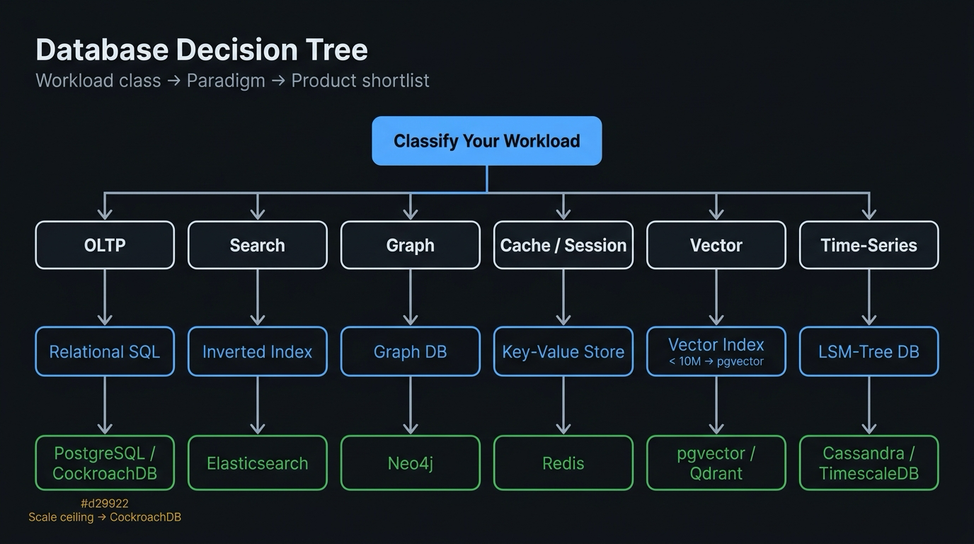
Summary
| Concept | Rule |
|---|---|
| Paradigm before product | Classify the workload before naming a product; the paradigm is the unit of decision. |
| Diagnostic checklist first | Run the diagnostic checklist first — most 'database problems' are application-layer problems in disguise. |
| Access pattern → paradigm | Access patterns (point lookup, scan, aggregation, graph) determine index strategy and therefore paradigm fit. |
| Consistency cost | Strong consistency is not free — it trades latency for correctness; choose it deliberately, not by default. |
| Polyglot cost | Polyglot persistence multiplies operational burden; a single store with extensions is superior at moderate scale. |
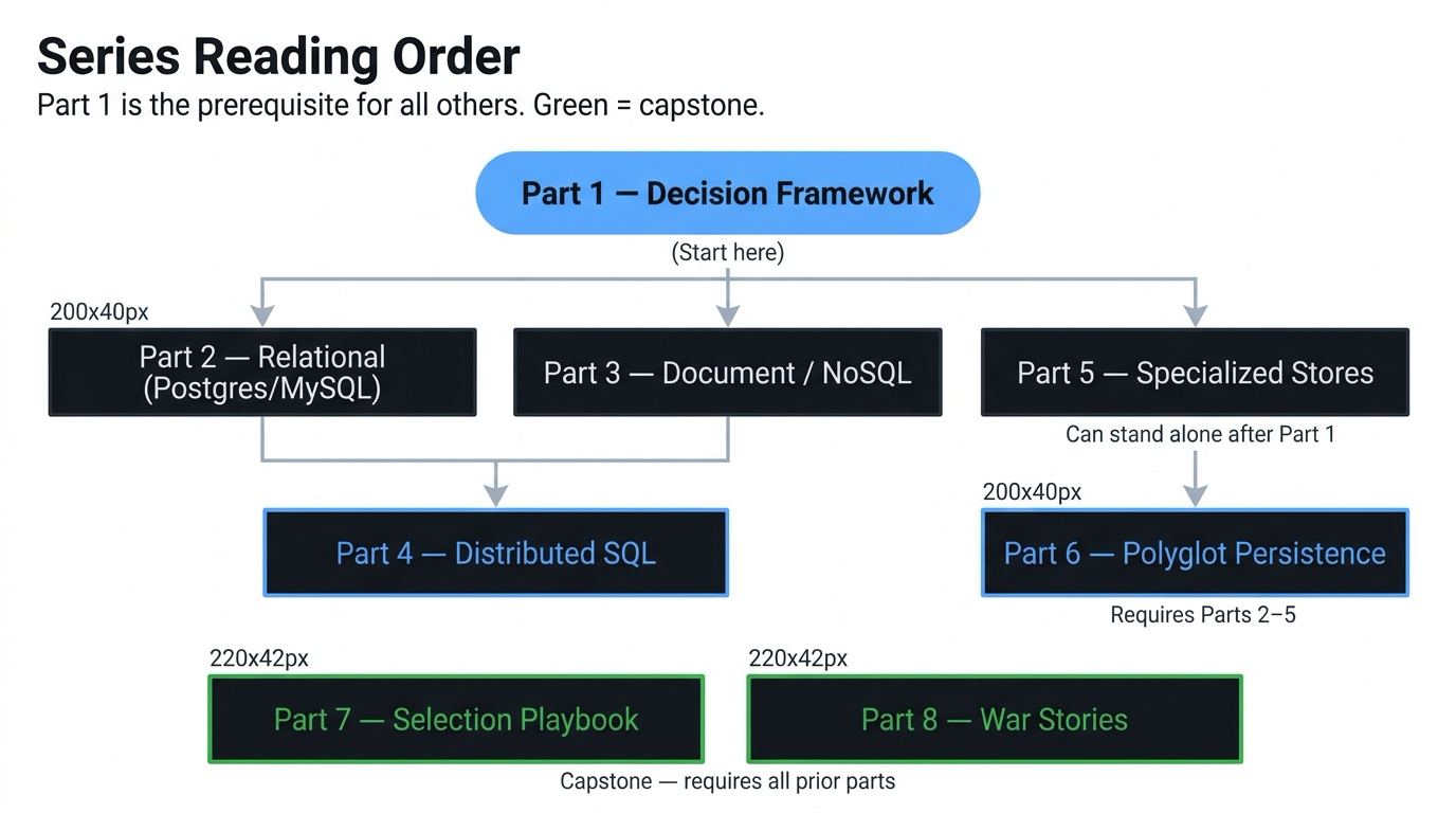
Related: Database Foundations Series — Every database paradigm decision begins with understanding the ACID/BASE trade-off. For the formal breakdown of each model, see ACID Database Properties: Atomicity, Consistency, Isolation & Durability in Practice and BASE Database Properties: Basically Available, Soft State & Eventual Consistency.
What's Next
In Part 2, we cover the relational paradigm in depth — PostgreSQL's extension model, MVCC under load, data modeling with JSONB, Row-Level Security for multi-tenancy, and the exact signals that tell you you've hit Postgres's ceiling.
This article was developed with AI-assisted deep search, specification cross-referencing, and technical research synthesis.