Database Internals: B-Trees, LSM Trees, WAL & Query Execution Plans
Every index, write-amplification tradeoff, and crash recovery guarantee your database makes is determined by its storage engine internals. This article maps B-Tree and LSM Tree mechanics to the production decisions you make daily — index design, WAL configuration, and reading EXPLAIN ANALYZE output like source code.
Advanced Database & State Management
Database Internals: B-Trees, LSM Trees, WAL & Query Execution Plans
A database is not a dumb storage box — it is a contract between your write path, your read path, and your consistency guarantees. Every design decision you defer becomes a production incident you eventually own. The most deferred decision in backend engineering is this: understanding what the storage engine is actually doing when you call INSERT, SELECT, or CREATE INDEX. Engineers who skip this layer add indexes until queries stop being slow, then wonder why write throughput collapsed. They disable fsync for performance, then lose data in a crash. They stare at EXPLAIN output and see words. This article closes that gap.
The canonical depth reference for this topic is Martin Kleppmann's Designing Data-Intensive Applications, Chapters 3 and 2. This article teaches the decision layer — the production choices that follow from understanding those internals. Read DDIA for theory; read this for Monday.
Series positioning: The Modern Database Paradigms series answers which database for which workload. This series answers why your database behaves the way it does inside the one you already chose. Read both — in either order.
1. B-Tree Internals: Why Adding Indexes Is Not Free
Every relational database you have ever used — Postgres, MySQL, SQLite — stores its indexes as a B-Tree by default. Understanding the B-Tree is not academic. It is the direct explanation for why a table with 20 indexes on it writes slower than one with 3, and why VACUUM is not optional.
1.1 Page Structure and Node Splits
A B-Tree organizes data into fixed-size pages (8 KB in Postgres). Each page is either:
- An internal node — holds fence keys and pointers to child pages
- A leaf node — holds the actual index entries (key + heap pointer)
When you insert a new row, the database walks the tree to the correct leaf page and inserts the key. If the leaf page is full, it splits: the page divides into two, and the parent internal node receives a new fence key pointing to the new sibling. If the parent is also full, the split propagates upward — potentially all the way to the root.
Index bloat compounds over time. Pages split on insert but never re-merge on delete. A table that has seen heavy churn accumulates half-empty pages — a phenomenon called index bloat — that inflates index size and slows scans. REINDEX CONCURRENTLY reclaims it without locking.
1.2 Fill Factor: The Write Buffer Inside the Page
Postgres lets you configure fillfactor per table or index (default: 100 for indexes, 100 for tables). A fillfactor of 70 leaves 30% of each page empty on initial fill. That empty space absorbs future inserts and HOT (Heap-Only Tuple) updates without triggering a page split.
Use fillfactor = 70–80 on indexes for columns that are frequently updated (status columns, counters, flags). Use the default 100 for append-only tables (event logs, audit trails) where rows are never updated.
2. LSM Tree Internals: The Write-Optimized Alternative
B-Trees are read-optimized: any key lookup is O(log n) with at most a handful of page reads. But their write path — which involves random page reads, in-place updates, and potential cascading splits — is a poor fit for workloads that are write-dominant with large data volumes.
Log-Structured Merge-Trees (LSM Trees) invert the tradeoff. They are used by RocksDB (the engine powering CockroachDB, TiKV, and PlanetScale), Cassandra, and LevelDB. Understanding them matters because engineers increasingly interact with these engines without realizing it.
2.1 The Memtable → SSTable Pipeline
LSM Trees operate in two tiers:
- Memtable (in-memory): incoming writes are appended to an in-memory sorted structure. Reads check the memtable first.
- SSTables (on-disk): when the memtable reaches a size threshold, it is flushed to disk as an SSTable — a sorted, immutable file. SSTables accumulate over time.
2.2 Write Amplification vs Read Amplification
The fundamental tradeoff between B-Trees and LSM Trees is measured in amplification factors:
| Metric | B-Tree | LSM Tree |
|---|---|---|
| Write amplification | Low (in-place update per page) | High (data written multiple times during compaction) |
| Read amplification | Low (O(log n) page reads) | Higher (may check multiple SSTable levels + bloom filter) |
| Space amplification | Low (pages reused) | Medium (stale versions live until compaction) |
| Sequential write throughput | Moderate (random I/O on splits) | High (all writes sequential) |
| Best workload | Mixed read/write, point lookups | Write-dominant, time-series, event ingestion |
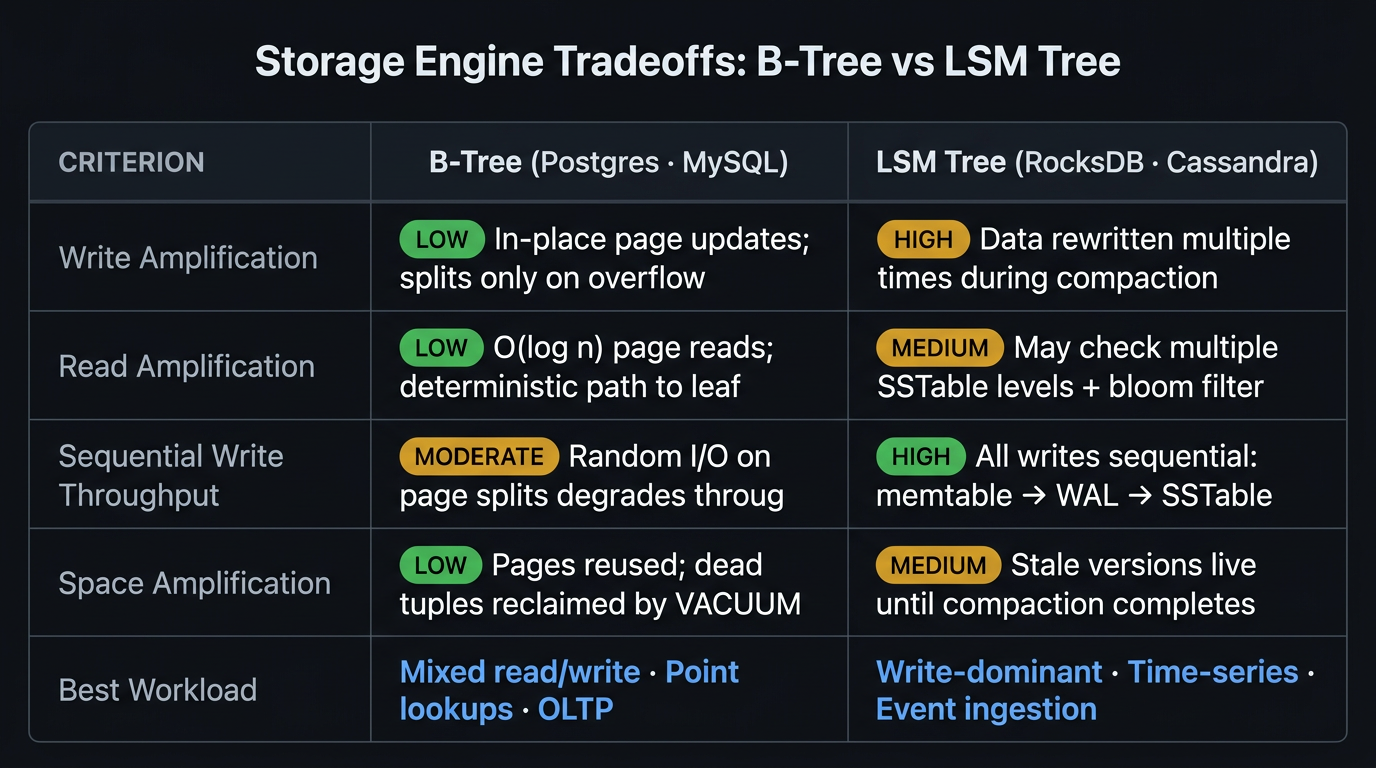
LSM Trees do not eliminate write cost — they defer it to compaction. During heavy compaction, read and write performance both degrade. Production RocksDB deployments tune compaction aggressively (max_bytes_for_level_multiplier, compaction_style) to prevent compaction storms from affecting p99 latency.
3. Write-Ahead Log (WAL): The Source of Atomicity
WAL works hand-in-hand with MVCC (Multi-Version Concurrency Control) — Postgres never overwrites a row in place, it appends new versions. This is why dead tuples accumulate and why VACUUM exists. If MVCC is new to you, read Relational Databases: PostgreSQL & MySQL in Production first — it covers MVCC at the concept level before you dig into the WAL mechanics here.
Every write to a Postgres table goes through the Write-Ahead Log before it touches the actual data file. This is not a backup mechanism. It is the primitive that makes transactions atomic and durable.
3.1 Anatomy of a WAL Record
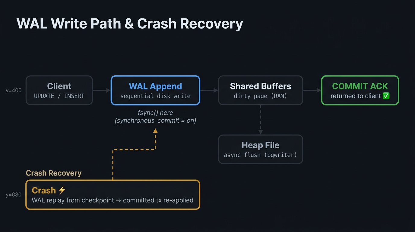
When you execute UPDATE orders SET status = 'shipped' WHERE id = 42, Postgres:
- Appends a WAL record to the WAL segment file on disk (sequential write — fast)
- Modifies the page in the shared buffer pool (in RAM — fast)
- The modified page is now a dirty page — it has not been written to the heap file yet
The dirty page is flushed to the heap file asynchronously by the background writer and the checkpoint process.
3.2 Crash Recovery: WAL Replay
If the server crashes between the WAL write and the heap file flush, Postgres recovers by replaying WAL records from the last checkpoint forward. Every committed transaction whose WAL record exists is replayed; every uncommitted transaction is rolled back.
This is why the WAL record must be written to durable storage before the commit acknowledgment is returned. The heap file state is always reconstructable from the WAL.
3.3 fsync and What Disabling It Actually Means
fsync = off tells the OS it may keep WAL writes in the OS page cache indefinitely — no guarantee they reach physical storage before a crash. A power loss or kernel panic in this state can corrupt the entire database cluster, not just lose recent transactions. This is not a latency tradeoff. It is a durability-off switch.
synchronous_commit = off is safer: it returns the COMMIT ACK before the WAL record is fsynced, risking loss of the last few committed transactions on crash — but without the cluster-corruption risk of fsync = off. Use it only where you can tolerate losing the last ~200ms of commits (e.g., analytics event ingestion, not financial transactions).
4. Query Execution Plans: Reading EXPLAIN ANALYZE Like Source Code
Most engineers EXPLAIN a query once, see "Seq Scan," add an index, and move on. The actual skill is reading the full EXPLAIN ANALYZE output and understanding why the planner made each decision — because the planner is sometimes wrong, and knowing when it is wrong is the only way to fix it.
4.1 EXPLAIN ANALYZE Output Anatomy
Key fields to read:
| Field | Meaning | When It Signals a Problem |
|---|---|---|
cost=X..Y |
Planner's estimated startup..total cost in arbitrary units | — |
rows=N (estimated) |
Planner's row count estimate from pg_statistic |
— |
actual time=X..Y |
Wall-clock time in milliseconds | High actual vs low estimated = planner surprise |
rows=N (actual) |
True row count from execution | Diverges greatly from estimated → stale stats |
loops=N |
How many times this node executed | loops > 1 on a Seq Scan = nested loop problem |
4.2 When Estimated ≠ Actual: The Planner Lies
This gap — estimated 12, actual 48,241 — means the planner's statistics are stale. It chose a Seq Scan because it thought the table had 12 matching rows, for which an index scan would be more expensive. With 48,000 rows, an index scan would have been dramatically faster.
The planner is a cost-based optimizer, not an oracle. Its estimates are only as accurate as its statistics. ANALYZE collects fresh statistics. EXPLAIN (ANALYZE, BUFFERS) shows buffer hit/miss counts — useful for diagnosing cache misses that inflate actual time.
4.3 Join Strategies: When the Planner Chooses Each
Postgres chooses between three join algorithms based on estimated input sizes and available memory:
| Strategy | How It Works | Best When |
|---|---|---|
| Nested Loop | For each outer row, scan inner relation | Inner relation is small OR indexed; outer is tiny |
| Hash Join | Build hash table from inner relation; probe with outer | Both relations large; no useful index on join key |
| Merge Join | Both inputs sorted on join key; merge in one pass | Both inputs pre-sorted (index exists on join key) |
5. Index Types Beyond B-Tree
The default CREATE INDEX creates a B-Tree. For many production access patterns, a more specialized index type delivers order-of-magnitude improvements.
5.1 Partial Indexes
A partial index indexes only rows matching a WHERE predicate. For tables where queries almost always filter on a status column with low cardinality (most rows are completed, queries almost always ask for pending), a partial index on the minority set is dramatically smaller and faster.
5.2 Covering Indexes
A covering index includes additional columns beyond the indexed key using INCLUDE. When all columns needed by a query are in the index, Postgres can answer the query from the index alone — an Index-Only Scan — without touching the heap file.
Index-Only Scans require the visibility map to be up to date. Run VACUUM regularly on tables with covering indexes to keep the visibility map current — otherwise Postgres falls back to heap fetches for visibility checks, defeating the covering index.
5.3 Expression Indexes
An expression index indexes the result of a function or expression. This is essential for case-insensitive searches and computed filters that appear in WHERE clauses.
6. Diagnosing Bloat: The Silent Table Decay
Postgres uses MVCC (Multi-Version Concurrency Control) — it never overwrites a row in place. An UPDATE writes a new row version and marks the old version as dead. A DELETE marks the row as dead. Dead rows accumulate until VACUUM reclaims their space.
CLUSTER reclaims table bloat and physically reorders rows by an index — but it acquires an exclusive lock for the duration. On large tables this means minutes of downtime. Use pg_repack (extension) for online reclustering without locks.
Summary
| Concept | Rule |
|---|---|
| B-Tree indexes | Every index is a write tax — add only indexes that appear in EXPLAIN output |
| Index fill factor | Use fillfactor = 70–80 on frequently-updated columns to absorb updates without splits |
| LSM Trees | Correct for write-dominant workloads; wrong for mixed read/write with point-lookup SLAs |
| WAL | The source of atomicity and durability — fsync = off disables durability, not just latency |
synchronous_commit = off |
Safe for tolerable data loss (analytics); never for financial or user-facing writes |
EXPLAIN ANALYZE |
Read estimated vs actual rows — divergence signals stale statistics; fix with ANALYZE |
| Join strategies | Wrong planner choice usually means stale stats or missing work_mem; fix the root cause |
| Partial indexes | Index only the minority set when queries almost always filter on a low-cardinality column |
| Covering indexes | INCLUDE extra columns to enable Index-Only Scans — requires up-to-date visibility map |
| Expression indexes | Index lower(email) not email for case-insensitive search patterns |
| Bloat | Dead rows accumulate via MVCC; VACUUM reclaims space; REINDEX CONCURRENTLY for indexes |
Related: Database Foundations Series — This article covers the physical storage engine that makes ACID possible. For the formal four-property ACID contract built on top of these WAL, buffer pool, and fsync primitives — see ACID Database Properties: Atomicity, Consistency, Isolation & Durability in Practice.
What's Next
In Part 2a, we build on the WAL atomicity foundation established here to examine isolation levels and concurrency control — the formal specification of which data anomalies your application is designed to tolerate, and the exact SQL that prevents each one. → Isolation & Concurrency Control
This article was developed with AI-assisted deep search, specification cross-referencing, and technical research synthesis.