Scaling Data: Partitioning, Sharding & Replication Strategies
Scaling data is a consistency and coordination problem, not a storage problem. This article covers table partitioning, sharding strategies and their irreversibility, and the write/read consistency tradeoffs of Master-Slave, Multi-Master, and Leaderless replication — including the quorum formula that makes leaderless replication safe.
Advanced Database & State Management
Scaling Data: Partitioning, Sharding & Replication Strategies
A database is not a dumb storage box — it is a contract between your write path, your read path, and your consistency guarantees. Every design decision you defer becomes a production incident you eventually own. The most expensive deferred decision in data architecture is sharding. Engineers reach for it when writes slow down — then discover it is irreversible, that cross-shard joins are now application code, and that cross-shard transactions are now Sagas. This article maps each scaling strategy to the consistency tradeoff it makes so you choose before you commit, not after.
This is Part 3 of the Advanced Database & State Management series. It builds directly on the consistency model vocabulary from Part 2b — Consistency Models & Distributed Coordination. Replication topology choices are meaningless without understanding what "consistent" means across replicas.
Cross-series reference: The Polyglot Persistence: When Multiple Databases Earn Their Cost article in the Modern Database Paradigms series covers CDC (Change Data Capture) via Debezium as the correct alternative to dual-write across multiple databases. If your sharding strategy requires cross-shard writes, Debezium-based CDC from a single source of truth is the pattern to use — not application-level dual-write.
1. Recognizing the Vertical Ceiling Before You Hit It
Before reaching for partitioning or sharding, verify you have actually hit the vertical scaling ceiling — not just the application layer's interpretation of it.
1.1 Signals That Precede the Actual Ceiling
| Signal | What It Means | First Fix |
|---|---|---|
| p99 write latency rising | Lock contention, index bloat, or buffer pool pressure | EXPLAIN ANALYZE, vacuum, index audit |
| Lock contention rate high | Too many writers competing for the same rows | Optimistic concurrency, smaller transactions |
autovacuum perpetually lagging |
Dead tuple bloat — MVCC accumulation exceeds vacuum throughput | Tune autovacuum_vacuum_cost_delay, dedicate a vacuum worker |
| Connection pool exhaustion | Too many application threads holding idle connections | PgBouncer transaction-mode pooling before sharding |
Checkpoint duration > checkpoint_completion_target |
WAL flush can't keep up with write rate | Increase max_wal_size, tune checkpoint_completion_target |
PgBouncer before sharding: Postgres struggles with connection count above ~500 active connections per node. PgBouncer in transaction mode multiplexes thousands of application threads onto a small pool of actual Postgres connections — eliminating a common "database is slow" symptom that has nothing to do with data volume.
2. Table Partitioning: Optimization, Not Scaling
Table partitioning divides a single logical table into multiple physical subtables (partitions). It is a query-optimization strategy — it does not distribute data across machines.
2.1 Partition Types
2.2 What Partitioning Removes
Partitioning and sharding are orthogonal strategies. Table partitioning is single-node. Sharding is multi-node. You can partition a table on a sharded node. Partition first to optimize queries; shard only when you exhaust the vertical limit of a single node.
2.3 The 5-Pillar Capacity Framework: Know Your Ceiling Before You Shard
Before escalating to sharding, you need to measure the actual ceiling of your current single node, not guess at it. Every database instance saturates in one of five physical dimensions. Identify which pillar is bottlenecking your system and you have a precise, quantified argument for — or against — sharding.
About the examples below. Each pillar is evaluated against the same concrete reference system: an AWS RDS db.t4g.micro (1 GB RAM, 2 Graviton2 vCPUs, 20 GB gp3 SSD) running PostgreSQL — a budget-tier instance typical of a low-to-medium traffic production service. The workload is an access-control event log: append-only inserts from ~10 concurrent connections at a burst of ~60 writes/sec during peak load.
These numbers are not benchmarks — they are worked examples of the formulas. Substitute your own instance specs (RAM, vCPU count, storage IOPS, connection pool size, average query latency) and the same arithmetic gives you your ceiling. The formulas are universal; the numbers change with your configuration.
Pillar 1 — Memory: RAM Saturation Point
A database instance either crashes with an Out-Of-Memory (OOM) error or degrades into slow disk reads the moment the active working set exceeds available RAM.
Example — db.t4g.micro (1,024 MB Total RAM):
- Saturation threshold: Exceed ~50 active connections → OOM restart risk.
- Verdict: Enforcing
maxConnections = 10in the application pool uses only ~80 MB of connection RAM — under 20% of the memory saturation limit. Headroom: 5×.
This formula is the correct justification for connection poolers like PgBouncer. The formula shows exactly how many raw connections your RAM can sustain; a pooler lets thousands of application threads share a small number of real Postgres connections that stay within this budget.
Pillar 2 — Concurrency: Little's Law (Throughput Ceiling)
How many operations per second (QPS) can the database process before connection queues build up?
Example — db.t4g.micro with a 10-connection pool:
- Saturation threshold: Connection queues start building above ~3,000 QPS.
- Verdict: A typical ferry-docking burst generates ~60 QPS — less than 2% of the concurrency ceiling. Headroom: 55×.
Little's Law is the reason query latency matters as much as connection count. Cutting average query latency in half (e.g., by adding an index) doubles your throughput ceiling without adding a single connection.
Pillar 3 — Disk I/O: IOPS Ceiling
Every database write causes Write Amplification: one logical row insert triggers multiple physical writes (WAL, B-Tree index updates, data block flushes). The disk IOPS budget must absorb all of them.
Example — AWS gp3 SSD with a 4-index table:
- Saturation threshold: Sustained writes above 500 writes/sec exhaust gp3 baseline IOPS.
- Verdict: At a burst of 60 writes/sec, disk I/O will not saturate. Headroom: 8.3×.
Reducing WAF is a more cost-effective lever than upgrading storage. Strategies: drop unused indexes (each index adds ~1 IOPS per write), use partial indexes, and ensure BRIN indexes instead of B-Tree where possible for time-series append-only data.
Pillar 4 — CPU: vCPU Processing Capacity
Example — db.t4g.micro (2 Graviton2 vCPUs):
- Saturation threshold: CPU only pegs at 100% when unindexed queries trigger full sequential scans across millions of rows.
- Verdict: With partition pruning and B-Tree indexes on all query paths, CPU usage stays below 5%.
A single SELECT * FROM large_table without an index clause launches a sequential scan that pegs a vCPU at 100% and blocks other queries. CPU saturation is almost always an index problem disguised as a hardware problem.
Pillar 5 — Contention: Row & Table Locks
Hardware resources are irrelevant if transactions block each other on locks.
Two common saturation triggers:
1. Hot-row lock contention — 50 concurrent writers all trying to UPDATE the same summary row.
2. DDL lock queuing — ALTER TABLE ... DETACH PARTITION requests an ACCESS EXCLUSIVE lock that blocks all incoming reads and writes.
Capacity Scorecard: Reading the Full Picture
Once you've evaluated all five pillars, produce a scorecard that compares your saturation limits against your actual peak usage. This is your evidence for — or against — sharding:
How to read this table: the column you care about is Headroom. If any dimension reads < 2× safe, that pillar is your imminent bottleneck — and is the only thing that warrants an infrastructure change. You do not shard because storage is large; you shard when the write-throughput or concurrency headroom drops below your growth runway.
The Active Hot Data row is the sneaky one. Even if total stored data is small, if your working set (the rows actively touched by queries in the last hours or days) exceeds shared_buffers, Postgres falls back to disk reads on every cache miss. This is the most common cause of a database "feeling slow" that has nothing to do with total row count or connection count.
The universal rule of thumb for a single-node Postgres instance:
A standard RDS db.t4g.micro comfortably handles any workload where all four of these are true simultaneously:
Violating any one of these four rules — not storage size, not total row count — is the signal to start planning a vertical upgrade or, as a last resort, sharding.
3. Sharding: The Irreversible Decision
Sharding distributes data across multiple independent database nodes (shards), each owning a subset of the data. It distributes write load across nodes — something partitioning cannot do.
3.1 Sharding Strategies
Range-Based Sharding
Advantages: Predictable placement, easy range queries within a shard. Disadvantage: Hot spots. If most active customers are in the 1M–2M range, Shard B gets all the write traffic. Rebalancing requires moving large contiguous ranges.
Hash-Based Sharding
Advantages: Even write distribution, no hot spots. Disadvantage: Range queries across the shard key require hitting all shards. Re-sharding (adding shards) invalidates all hash assignments — requires full data rehash or consistent hashing (minimizes remapping on node addition).
Directory-Based Sharding (Consistent Hashing)
Advantages: Most flexible, supports heterogeneous shards, minimizes remapping on rebalance. Disadvantage: Router service is a single point of failure; routing table must be highly available.
3.2 The Operational Contract You Sign
Sharding is effectively irreversible. Once you shard:
- Foreign key constraints across shard boundaries disappear — referential integrity is now your application's problem.
- Cross-shard transactions must be replaced by Saga patterns — 2PC across shards is operationally fragile.
- Re-sharding (changing shard count) requires dual-write migration or a full rebuild — plan the initial shard count for 3–5× current volume.
- Every new database feature evaluation must account for sharding compatibility.
4. Replication Topologies
Replication copies data from one node to one or more others. Unlike sharding, replication duplicates data — each node has the same data. This provides read scalability and fault tolerance, not write scalability.
4.1 Master-Slave (Single Primary)
- Writes: Primary only. All write capacity is limited to one node.
- Reads: Distributed across replicas — scales read throughput linearly with replica count.
- Consistency: Replicas lag behind primary. Reads from replicas may be stale.
- Failover: Promote a replica to primary. Manual or automatic (Patroni, repmgr).
4.2 Multi-Master (Active-Active)
- Writes: Any primary accepts writes simultaneously.
- Conflict: Concurrent writes to the same row on different primaries → conflict.
- Resolution strategies:
- Last-Write-Wins (LWW): timestamp determines winner — silently discards the loser.
- Application-level merge: application receives both versions and merges.
- CRDTs: automatic conflict-free merge for compatible data types.
Multi-master LWW conflict resolution silently discards writes. This is not a configuration option — it is the logical consequence of accepting concurrent writes to the same row on different nodes with no distributed lock. For any data where concurrent writes have semantic meaning (balances, counters, inventory), you need application-level conflict detection or CRDTs.
4.3 Leaderless Replication (Dynamo-Style)
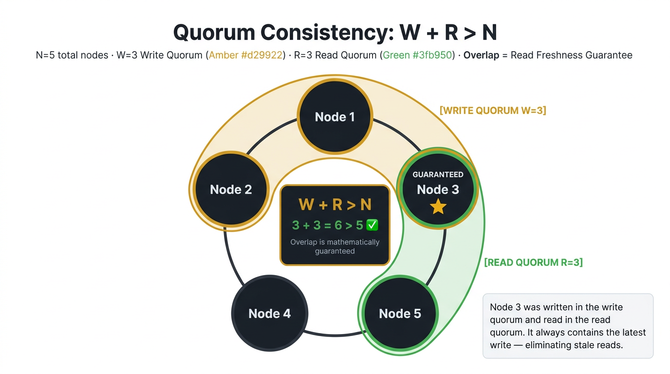
There is no designated primary. Any node accepts both reads and writes. Consistency is achieved through quorum.
5. Replication Topology Decision Matrix
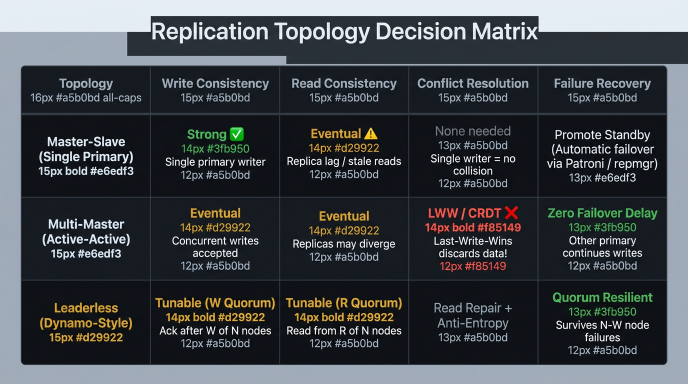
| Topology | Write Consistency | Read Consistency | Conflict Resolution | Failure Recovery |
|---|---|---|---|---|
| Master-Slave | Strong (single writer) | Eventual (replica lag) | None needed (single writer) | Promote replica (minutes) |
| Multi-Master | Eventual (concurrent writers) | Eventual | LWW / app merge / CRDT | No failover needed (other primary continues) |
| Leaderless | Tunable (W quorum) | Tunable (R quorum) | Read repair / anti-entropy | No failover (surviving nodes maintain quorum) |
6. Logical vs Physical Replication
Postgres offers two replication modes with different use cases:
| Dimension | Physical Replication (WAL streaming) | Logical Replication (row-level events) |
|---|---|---|
| What is replicated | Raw WAL bytes — byte-for-byte identical copy | Row-level INSERT/UPDATE/DELETE events |
| Cross-version | ✗ — same major version only | ✅ — different Postgres major versions |
| Selective tables | ✗ — entire cluster | ✅ — subscribe to specific tables |
| CDC pipelines | ✗ — not suitable | ✅ — feed Debezium/Kafka with row events |
| Blue-green migration | ✗ — full cutover required | ✅ — run old and new side-by-side |
| Replica usage | Read-only standby | Can write to non-subscribed tables |
Use logical replication for zero-downtime Postgres major version upgrades and for feeding CDC pipelines (Debezium → Kafka). Use physical replication for standby high-availability replicas and PITR backup targets. The two can coexist on the same Postgres primary.
Summary
| Concept | Rule |
|---|---|
| Vertical ceiling signals | Check p99 latency, lock contention, connection pool exhaustion, and vacuum lag before reaching for sharding |
| PgBouncer first | Connection pool exhaustion is a common "database is slow" symptom that PgBouncer solves before sharding is needed |
| Table partitioning | Query optimization on a single node — not distributed scaling; enables cheap time-window archival |
| 5-Pillar capacity framework | Measure all five pillars (Memory, Concurrency, I/O, CPU, Contention) before deciding to shard — headroom < 2× on any pillar is the signal to act |
| Sharding | Distributes write load; is irreversible; cross-shard joins become application joins; plan shard count for 3–5× current volume |
| Co-location | Shard related entities on the same key so joins stay within a single shard |
| Master-Slave | Strong single-writer consistency; read replicas lag — route consistency-required reads to primary |
| Multi-Master LWW | Silently discards concurrent writes — never use for financial or user-generated content |
| Leaderless quorum | W + R > N guarantees at least one overlapping node has the latest write |
| Logical replication | Required for cross-version upgrades, CDC pipelines, and blue-green migrations |
| Physical replication | HA standby and PITR backup — byte-identical copy, same Postgres version only |
Related: Database Foundations Series — The leaderless replication, quorum formula (W + R > N), and anti-entropy patterns covered here are the mechanical implementation of the BASE model. For the formal BASE paradigm — Basically Available, Soft State, and Eventual Consistency — see BASE Database Properties: Basically Available, Soft State & Eventual Consistency.
What's Next
Part 5 brings this series to the application layer: ORM Internals — the N+1 problem, why lazy loading fires N SQL queries invisibly, and how the DataLoader pattern is the minimum correct implementation for any list-loading path. → ORM Internals: N+1, Lazy Loading & Eager Loading
This article was developed with AI-assisted deep search, specification cross-referencing, and technical research synthesis.